|
|
|


Looking
at Data in 10 Minutes#1
Overview
This is Part 1
of 3 for what you might find in a typical Intro to Probability and Statistics
course.
This covers
Mean, Median, Mode, Variance and Standard Deviation, Frequency Distributions
and Histograms
Click this
link for Part 2: Probability in 10
Minutes
Click this
link for Part 3: Statistics in 10
Minutes
Who Is This For?
Someone without any prior experience, such as a college freshman
about to take her first Statistics class.
Key Goals for
Each of the 3 Parts
1) Introduce
the Concepts, Terminology and Symbols that would be
covered in a typical Intro to Statistics course.
2) Provide an intuitive understanding
of things versus just providing formulas.
3) Present the
information step-by-step in the
best order for learning.
Looking at Data
Part 1: Mean, Median and Mode
1) Mean: This is short for the Arithmetic
Mean#2.
1.1) The Mean is the average of a set of numbers#3.
1.2) The formula is to sum up all values and divide by the total
number of values#4.
1.3) The number of values is typically written as N for ‘Number’. Uppercase ‘N’.
1.4) We’ll
write out the values as x1
for the first value, x2
for the second value and so on, all the way up to xn for the last value
with a lowercase ‘n’.
1.5) The Mean is typically written using Greek
letter mu, which is µ
1.6) The uppercase Greek letter sigma which looks like this ∑
is typically used to mean ‘the sum of’.
1.7) We will therefore write the formula for the Mean as:
µ = x1 + x2 + x3
+ ... + xn / N
or as:
µ = ∑x / N
1.8) As an example, the Mean
of these 3 numbers is 105.333333:
Number 1) 110
Number 2) 98
Number 3) 108
µ = (110 + 98 + 108) / 3
µ = 105.333333
1.9) The Mean of the values on a 6-sided die
(singular of dice) is:
µ = (1 + 2 + 3 + 4 + 5 + 6) / 6
µ = 3.5
1.10) Observe
that the mean does not need to be one of the source numbers. The Mean of 3.5 is not one of the vales on
a die.
1.11) For the Mean, the order of the numbers does not
matter.
The
Arithmetic Mean of this set of numbers:
110, 98, 108
Is the same as
the Arithmetic
Mean of this (same) set of numbers (written in a different order):
98, 108, 110
1.12) Excel
function to use is ‘AVERAGE’
2) Median:
This is the middle number in a set of numbers. This requires that you order the numbers from
smallest to largest.
2.1) For example,
for this set of 5 numbers, the Median
is 8.
Number 1) 1
Number 2) 8
Number 3) 8
Number 4) 9
Number 5) 9
By comparison,
the Mean is:
µ = (1 + 8 + 8 + 9 + 9) / 5
µ = 7
2.2) Since the Median
is just the middle number, in this example the Median would still be 8.
Number 1) -101
Number 2) 2
Number 3) 8
Number 4) 55
Number 5) 999
In the prior
example, the Mean was 7, which is
pretty close to the Median of
8. In this example, the Mean is intentionally very different to
illustrate the point. The Mean here is
192.6.
2.3) The Median is used instead of the Mean in cases where a small number of
very large values (or very small values) can Skew things one way or another.
The most
common example is looking at incomes, how much money people earn in a
year.
For example,
if you have a room of 11 people with 10 average earners and Elon Musk (one of
the richest people in the world), the Arithmetic Mean of their incomes, which
would include Elon’s, might be over a million dollars. While their Median income, which is the income of the 6th person,
ranked from least income to most income, might be $50,000, well under the
average of $1m.
2.4) Excel
function to use is ‘MEDIAN’
3) Mode:
This is the most common number in a set of numbers#5.
As with the Mean, the order of the numbers does not
matter in determining the Mode. Although ordering the numbers is not a
requirement, we’ll present the numbers ordered from lowest to highest to make
it easier to see the most common numbers.
3.1) For this example of 6 numbers, the Mode is 9. The number 9
repeats 3 times, more than any number.
Number 1) 1
Number 2) 8
Number 3) 8
Number 4) 9
Number 5) 9
Number 6) 9
Alternately, we
can write this set of numbers as a list like this:
1, 8, 8, 9, 9, 9
3.2) If there are two numbers that repeat the same number of
times and especially if they are non-adjacent the set of numbers is sometimes
called ‘Bimodal’.
For example, this
set of 10 numbers is Bimodal with Modes of 2 and 9.
1, 2, 2, 2, 6, 8, 8, 9, 9, 9
3.3) Excel
function to use is ‘MODE’.
Looking at Data
Part 2: Variance and Standard Deviation
1) Variance: A measure of variation or variability of a
set of numbers. This is a hugely
important concept in many areas such as finance and accounting.
Examples:
1.1) In
finance, a stock or that has a bond that range of values is considered less
risky than one that has a larger range of values.#6
1.2) In
manufacturing, if you need to make a metal bar exactly one meter long, a
machine that makes them 0.999 to 1.001 meters long (small variation) will be
better than one that makes them 0.98 to 1.02 meters long (larger
variation). This is especially important
when you are making many pieces that need to fit together, like parts of a car.
2) Standard Deviation: This is another
measure of variation or variability of something. This is related to the Variance. The Standard
Deviation is defined as the square root of the variance.
3) In practice
sometimes the Standard Deviation
will be used and sometimes the Variance
will be used. For the examples above for
finance and manufacturing, the measurement of variation are more commonly
presented as Standard Deviations. You might see the Variance used in some
formulas in Statistics.
The point is
to make sure which one you are working with in any particular context. Of course, if you have one of them, you can
easily get the other by either squaring the value or taking the square root, as
appropriate.
4) Symbols#7:
4.1) Variance: The symbol is the lowercase
Greek letter sigma squared: σ2
4.2) Standard Deviation: The symbol is the
lowercase Greek letter sigma (without the squared): σ
5) Formulas
5.1) The Variance of a population is the Average of the Squared Deviations from the Mean.
We’ll write
that out as#8:
σ2 = [(x1
- µ)2 + (x2 - µ)2 + (x3 - µ)2 + … + (xn - µ)2] / N
Remembering
that:
x1 = the
first value
xn = the
last value. Lowercase ‘n’
µ = the Mean, i.e., the Arithmetic Mean
N = the total number of values.
Uppercase ‘N’.
5.2) The Standard Deviation is just the square
root of that.
We’ll write
that as either this:
![]()
Or like this,
which is a bit easier to do on a computer:
σ = ( [(x1 - µ)2 + (x2 - µ)2 + (x3 - µ)2 + … + (xn - µ)2] / N )^1/2
6) Example:
Variance of a Die (Single of Dice).
Values are 1, 2, 3, 4, 5, 6.
N, the number of values, is 6.
Step 1) Figure out the Mean. As previously shown:
µ = (1 + 2 + 3 + 4 + 5 + 6) / 6
µ = 3.5
Step 2) Use
this Formula for Variance.
σ2 = [(x1 – 3.5)2 + (x2
- 3.5)2
+ (x3 - 3.5)2
+ (x4 - 3.5)2
+ (x5 - 3.5)2
+ (x6 - 3.5)2]
/ 6
σ2 = [(1 – 3.5)2 + (2 - 3.5)2 + (3 - 3.5)2 + (4 - 3.5)2 + (5 - 3.5)2 + (6 - 3.5)2] / 6
σ2 = [(–2.5)2 + (–1.5) 2 + (–0.5)2 + (+0.5)2 + (+1.5)2 + (+2.5)2] / 6
σ2 = [6.25 + 2.25 + 0.25
+ 0.25 + 2.25 + 6.25] / 6
σ2 = 17.5 / 6
σ2 = 2.916667
6.25
2.25
0.25
0.25
2.25
6.25
Step 3) And then take the square root to calculate the Standard Deviation.
σ = 2.916667^1/2
σ = 1.707825
7) Excel
functions to use depending on your version of Excel are:
For Variance:
=VARP(A1:A6)
or
=VAR.P(A1:A6)
For Standard
Deviation:
=STDEVP(A1:A6)
or
=STDEV.P(A1:A6)
Notes:
7.1) The ‘P’ in the function names is for Population. There are similarly named
functions, e.g., STDEV (without the ‘P’) which will be used later when we
discuss topics on Statistics. The
formulas are slightly different.#9
7.2) The Excel
functions were given assuming that the data was located in Cells A1 to A6. You’ll need to vary those values for your
data as appropriate.
Looking at Data
Part 3: Frequency Distributions
1) Frequency Distribution: A table of data showing counts (frequencies)
of numbers for single numbers or for a range.
2) Example
We’ll look at
the count of the sum of 2 dice. Each die
has values 1 to 6 which allows for the sum ranging from 2 to 12.
We’ll use this
notation (Dice1, Dice2) to show the values.
For example, if Dice1 is a 2 and Dice2 is a 5, that
would look like this:
(2, 5)
Importantly,
if Dice1 is 5 and Dice2 is 2, then that would look like this:
(5, 2)
In other words
(2, 5) and (5, 2) are considered different, even though they both sum up to 7. Using this approach there are 36 possible
variations for 2 dice.
Here are the Sum of Two Dice with details shown for sums from 2
to 7:
Sums to 2:
Frequency = 1
(1, 1)
Sums to 3:
Frequency = 2
(1, 2), (2, 1)
Sums to 4:
Frequency = 3
(1, 3), (3, 1),
(2, 2)
Sums to 5:
Frequency = 4
(1, 4), (4, 1),
(2, 3), (3, 2)
Sums to 6:
Frequency = 5
(1, 5), (5, 1),
(2, 4), (4, 2), (3, 3)
Sums to 7:
Frequency = 6
(1, 6), (6, 1),
(2, 5), (5, 2), (3, 4), (4, 3)
Sums to 8:
Frequency = 5
Sums to 9:
Frequency = 4
Sums to 10:
Frequency = 3
Sums to 11:
Frequency = 2
Sums to 12:
Frequency = 1
3) Classes: Classes are the number of groupings for a
Frequency Distribution. Other terms for this concepts are ‘Ranges’
or ‘Buckets’.
For the prior
example of the sum of two dice, there are 11 Classes, ranging from 2 to 12.
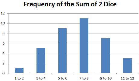
If we wanted,
we would reduce the number of classes from 11 down to just 6, with values based
on ranges like this:
Class1: Dice
Sum to 1 to 2: Frequency = 1
Class2: Dice
Sum to 3 to 4: Frequency = 5
Class3: Dice
Sum to 5 to 6: Frequency = 9
Class4: Dice
Sum to 7 to 8: Frequency = 11
Class5: Dice
Sum to 9 to 10: Frequency = 7
Class6: Dice
Sum to 11 to 12: Frequency = 3
See that if
you sum up the frequencies, you get the same total of 36.
36 = 1 + 5 + 9
+ 11 + 7 + 3
Looking at Data
Part 4: Histogram
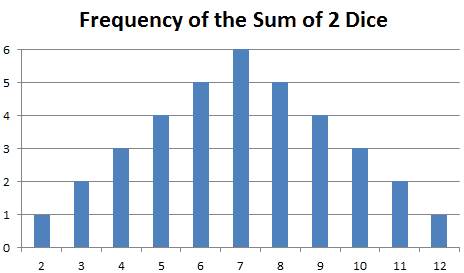
1) Histogram: A graphical representation of a Frequency
Distribution
2) Examples
Example 1
Based on the original example of the sum of 2 dice.
The Y-axis is the
count. The X-axis is the Class.
For example,
see the bar in the lower left. That
shows that there is 1 case when dice sum to 2.
In the middle it shows there are 6 cases when dice sum up to 7.
See that the
total number of possible sums of 2 dice is still 36 even when viewed as a
graph.
Example 2
This is based
on the 2nd example of having 6 Classes for the Sum of 2 Dice Rolls.
3) Looking at
Histograms, Mean, Median and Mode
Typical for
Intro to Statistics classes you be asked to look at a Histogram and answer
questions about the Mean, Median and Mode.
We’ll provide
the frequencies here in table form (Frequency Distribution), though for a test
you’ll likely just get the Histogram.#10
|
Range |
Frequency |
|
1 to 10 |
4 |
|
11 to 20 |
8 |
|
21 to 30 |
15 |
|
31 to 40 |
25 |
|
41 to 50 |
43 |
|
51 to 60 |
63 |
|
61 to 70 |
75 |
|
71 to 80 |
62 |
|
81 to 90 |
41 |
|
91 to 100 |
31 |
That totals to
367 different values:
367 = 4 + 8 +
15 + 25 + 43 + 75 + 62 + 41 + 31
Histogram:
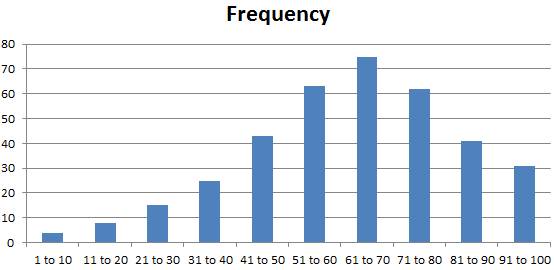
Questions:
Q1) What is the Mode?
A1) This is typically the easiest to discern. This is the number or range of numbers that
has the highest frequency. In this case,
that is the range from 61 to 70, which has a total of 75 values within that
range.
Q2) Which is higher, the Median
or the Mean?
A2) This is a bit harder to figure out just by looking at the
above Histogram. We’ll show a trick on
how to figure this out.
As a reminder,
the Median is the middle value,
ranked from smallest to largest. There are
367 values in total, so the middle value would be the 184th number. Although we are not going to
use that directly here.
For the trick,
we start by observing the values are skewed to the left. Then we can create a smaller set of values
that we can more easily wrap our heads around.
Let’s use
these 5 value values:
1, 8, 8, 9, 9
That looks
like this as a Histogram. This is also
skewed to the left though somewhat simplified.
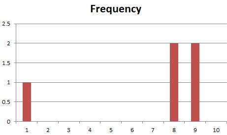
The Median is 8, as that is the middle
number, the third of the 5 numbers:
1, 8, 8, 9,
9
For the Mean, we have:
µ = (1 + 8 + 8 + 9 + 9) / 5
µ = 35 / 5
µ = 7
The answer in
this case is the Mean is less than
the Median, which will be true for Distributions that are skewed to the left.
For
distributions that are skewed to the right, that would be reversed and the Mean would be higher than the Median.
Example data:
1, 1, 8, 8,
9
Median: 8
Mean: 5.4
The key here
is that you may be asked this question just by looking at a Histogram and
without having access to the underlying table of data.
Footnotes
#1) The title of this page was inspired by ‘Learn Python in 10
Minutes’ at:
https://www.stavros.io/tutorials/python/
#2) Another ‘mean’ is the ‘Geometric Mean’. That has a formula
where you multiply all of the numbers and then take the square root. For example, for these three numbers which
represent the assumed returns on a stock for three years:
Year 1: 110%
Year 2: 98%
Year 3: 108%
We are writing
this to show the ending value relative to the starting value, so by 110% we
mean that the stock went up 10%. And for
98%, we mean that the stock went down 2%.
This is called
the ‘one plus’ approach, since we are adding one to
the return. i.e., take -2% and add one
and get +98%.
This makes the
math nicer for Geometric Means because we don’t need to worry about negative
numbers, since we are assuming stock prices can’t go below zero.
For the above
example, we get this Geometric Mean:
Geometric Mean
= (110% * 98% * 108%)^1/3
Geometric Mean
= (116.42400%)^1/3
Geometric Mean
= 105.19962%
Compare that
to the Arithmetic Mean of 105.33333%, which is just summing the numbers and
dividing by 3.
#3) The Mean
is the ‘Simple Average’ of a set of numbers.
There is another kind of average called the ‘Weighted Average’, which
each of the values you are averaging is given a weighting other than 1/n.
#4) While it
is not important for now, try to remember for later that the concept of the
Mean (Arithmetic Mean) applies only when we have a set of numbers
which represent the complete set of things.
The term for this is ‘Population’. The average of a Population is known as the
Mean and we use the symbol µ.
When we are
working with a Sample of data, there
is a different term used for the average and a different symbol. The term is Sample Mean and the symbol is an
x with a bar over it: ![]()
Sample Mean = ![]()
An example of
a sample would be to pick 10 students at random from a class of 30 and take
their average height. The Sample Mean
would be the average of the 10 selected students. In the Statistics Part, we’ll show how to use
Statistical
Inference to Estimate the Population Mean of the overall
population of 30 students and provide a range around it called a Confidence Interval where we can be 95%
sure, based on some assumptions, that the true Population
Mean of the 30 students is within that range.
#5) The Mode as a value is as a practical
matter used far less than the Mean
or the Median. The Mean is by far the most used and so most
important concept to know.
#6) For stocks, bond and commodities, finance professionals
typically measure the change in values from one do to another when determining
how risky a something is. For
simplicity, we’ll say they use the percentage change. Finance professionals will use the term
‘Volatility’ to describe the Standard
Deviation of the percent price
change on an annualized basis.
Examples:
6.1) A stock
that trades $100
one day, then $110 the next and then $105 on the third day has day-over-day
percentage moves of up 10% and then down 4.5%.
That is
considered less risky than a stock that trades like this:
6.2) $4 on day 1, $5 on day 2 and $4.25 on day 3.
Those percentages are much higher.
25% up move from Day 1 to Day 2 and 15% down move from Day 2 to Day 3.
#7) While it is not important for now, try to remember for later
that the symbols σ2
for Variance and σ for Standard
Deviation are to be used only when talking about Population, meaning the
complete set of numbers. The term for
this is ‘Population’.
When we are
working with a Sample of data, there
is a different symbol used. For a Sample
of Data, we use lowercase s for Standard
Deviation and then square it for Variance.
Variance of a Sample: s2
Standard Deviation of a Sample: s
#8) This formula for Variance
should be used only when working with a Population,
meaning you know all of the possible values.
When dealing with a Sample of data from a bigger Population, there is a slightly different formula. That will be discussed in the Statistics section. As a comparison, the formulas for Arithmetic Mean (of a population) and Sample Mean are basically the
same. The formulas only diverge when we
get to Population Variance versus Sample Variance.
8.1) Some may wonder why we take the square of the
difference. That is to get rid of
negatives. Suppose we just took the
average of the differences for each value from the mean. Without the squaring. That would look like this using the single
die as an example:
??? = [(x1 – 3.5) + (x2 - 3.5) + (x3 - 3.5) + (x4 - 3.5) + (x5 - 3.5) + (x6 - 3.5)] / 6
??? = [(1
– 3.5) + (2 - 3.5) + (3 - 3.5) + (4 - 3.5) + (5 - 3.5) + (6 - 3.5)] / 6
??? = [(–2.5)
+ (–1.5) + (–0.5) + (+0.5) + (+1.5) + (+2.5)] / 6
??? = 0 / 6
??? = 0
An average
deviation of 0 (zero) would not make much sense.
An alternate
approach might be to take the average of the absolute value of the differences.
Average Deviation = [abs(x1 – 3.5) + abs(x2 -
3.5) + abs(x3 -
3.5) + abs(x4 -
3.5) + abs(x5 -
3.5) + abs(x6 -
3.5) ] / 6
Average Deviation = [abs(1 – 3.5) + abs(2 - 3.5) + abs(3 - 3.5) + abs(4 - 3.5) + abs(5 - 3.5) + abs(6 - 3.5)] / 6
Average Deviation = [2.5 + 1.5 + 0.5
+ 0.5 + 1.5 + 2.5] / 6
Average Deviation = 9 / 6
Average Deviation = 1.5
A value of 1.5
is more reasonable. That said, we won’t
be saying anything more about the Average
Deviation as it is rarely used relative to the Variance and the Standard
Deviation.
#9) See this link for an explanation of the difference in the
formulas for the Population Variance
versus the Sample Variance. Note: When we say ‘Sample Variance’ we really mean to say that we are using the data
from a Sample to derive an Unbiased
Estimator of Population Variance
for the overall Population from
which we took the samples.
Link: Population Variance versus
the Sample Variance
#10) Looking
at the Frequency Distribution and looking
at the first class, which is for values ranging from 1 to 10, a note that we
don’t know exactly what those values are.
They could be:
1, 1, 5, 6
Or
7, 8, 8, 9
Or non-whole
numbers like
1.5, 6.5,
7.343, 8.9
All we know
about them is that there are 4 of them and they are greater or equal to 1 and
less than or equal to 10.