|
|
|


|
Main Page for Subject Area |
||
MTM Explained
1) MTM
Definition
MTM (Mark-to-Market) is the value of a trade. It is sometimes called the present value, meaning the value as of today. There is also a concept of ‘future value’ meaning the value of a trade at a future point in time.
2) Present
Value / Future Value formula
Future value answers questions like this… If you put $100 in the bank today at 5% interest, how much will you have in a year? The answer is… you’ll have $105 which is your original $100 plus $5 interest.
Turning that around, you could ask, how much would need to put into the bank to get $105 in a year? And the answer would be $100. The $100 is the present value and the $105 is the future value. Note that there is only 1 present value. There are many future values, one for each day in the future.
If we want to know what is the present value of $100 for one year from now
(instead of the $105 in the example above)… then we can calculate the ratio of
the numbers above:
$100 / $105 = 0.9523809524
That ratio is a value between 0 and 1.00 and it is called the ‘discount factor’
so we can express the above as:
Present Value / Future Value = Discount Factor
and we can rearrange those terms as
Present Value = Future Value * Discount Factor
and use that formula and that ratio to calculate the present value of $100 one year from now (rounded to two decimal places):
$95.23 = $100 * 0.9523809524
3) Compounded
Interest
The above example assumes simple interest, which in this context just means one interest payment at the end of the year. However, we could make the example more complicated by assuming two interest payments per year, i.e., one every 6 months. This is sometimes called ‘compound interest’ because the interest from the first payment (after 6 months) is ‘compounded’ , meaning that the second payment (the one after 12 months) includes interest both on the original amount (which is sometimes called the ‘principal’ amount) and the interest from the first six months.
For example, if you start with $100 and earn interested of 5% compounded semi annually (every 6 months) you get this:
Time Now: $100
Time 6 months: $102.50
This is your original $100 plus half of the 5% interest that you are due to get each year.
Time 12 months (one year): $105.0625
This the $102.50 you has after 6 months, plus another $2.50 in interest on the original $100 plus interest of $0.0625 on the $2.50 of interest you received after 6 months. Note that if you took the $2.50 of interest after the first six months out of the bank and spent it, then you would have only $105 after a year. The effects of compounding interest are seen only if you keep your money in the bank and earn interest on your interest.
If you increase the frequency of the compounding and keep your money in the bank… you get 105.1162, which is more than then $105.0625 you get from just 2 interest payments a year.
4) Interest
Rate Examples
Here is a table with examples of how much you would have if you put your money in the bank for one year based on different rates of compounding. For example, if you earn 3% per year and there are payments every 6 months, that is 2 payments, so $100 put in the bank under those terms would result in a value of $103.0225 after a year.
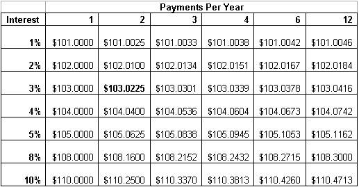
Click here to view this as a table (i.e., not as a picture)
And here is the same table expressed as discount factors, which are the ratio of present value divided by future value:
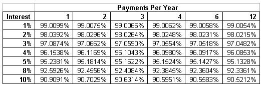
Click here to view this as a table (i.e., not as a picture)
5) Yield Basis
To more accurately compute the discount factor you would need to better determine the number of days on which you are earning interest. For example, whether there are 28, 29, 30, or 31 days in a given month. Holidays vs. good business days and leap days (i.e., Feb 29 during a leap year) can also play a role. Sometimes, you may need to calculate interest payments assuming actual days and sometimes you may need to calculate interest assuming you get the same payment for each month, i.e., you ignore the actual number of days in the month. A term commonly used to describe what is known as the ‘day count’ logic is ‘Yield Basis’. An example yield basis is 30 / 360, which means use the same time to compute interest for each month. I.e., 30 days for 12 months makes a pretend 360 days in the year. Another example yield basis is Actual / Actual which means use actual days.
6) MTM for a
Commodity Swap
A ‘Commodity Swap’ is a trade where two counterparties agree to make payments to each other for one or more months based on the price of some commodity. A Commodity Swap is an example of a type of trade called a ‘derivative’ because the value (i.e., the MTM) of a swap is derived (hence the term derivative) from the price of some underlying commodity.
A typical example might be where one firm agrees to pay $80 per barrel for 1000 barrels of crude oil for three months, e.g., January, February, and March to another firm. And suppose the other firm might agree to pay the first firm the value of the crude oil per barrel for 1000 barrels. The value per barrel to be paid would be determined at a future date. It would need to be determined by some impartial third party, because it wouldn’t be fair to allow one firm to set the price. A typical third party (third party just means that the organization is not one of the two parties directly involved in the swap agreement, i.e., not one of the two parties with a direct interest because they have to make payments. The payments would be made each month and since there are three months (January, February, and March) that means 3 payments. The work ‘payment’ is used to mean a cash flow, i.e., a payment, and it is also used to mean a receipt of cash. The payments would typically be a few days after the price per barrel is determined, meaning finalized. E.g., Five business days after the price determination date.
Notes:
1) This type of trade is called a ‘Fixed/Float’ or ‘Fixed for Float’ Swap, or sometimes a ‘Fixed for Float Financial Swap’. The fixed refers to the fixed payment, in this case the payment will be $80/ barrel for 1000 barrels, or 3 payments (one per month) of $80,000. The ‘float’ refers to the payments that are said to ‘float’, meaning that they are unknown / undetermined at the time of the original trades.
2) The time frame from this example trade is sometimes called a Jan – Mar swap (pronounced Jan to March swap or Jan through March swap) or a Q1 swap where Q1 means quarter one, meaning January to March. Cal 2012 would mean a calendar year swap, typically with monthly payments, January to December in 2012.
3) The above example deal is entirely cash settled. In other words, no physical commodity changes hands, i.e., no crude oil is actually delivered.
4) Typically the payments are netted out and so only one of the counterparties would pay the difference in payment, i.e., whoever owes the most. In other words, instead of one counterparty paying $80,000 and the other paying the first $81,000… the second counterparty would just pay the first the net of $1,000 and the first party, the one who originally owned $80,000 would not have to make a payment. This concept, known as ‘netting’ reduces the credit risk from one party to another.
A typical arrangement is for the dates for determining the price to be paid per barrel on the floating side of the swap are based on the last day of trading for the relevant contract month from the commodities exchange. Unlike the swap in this example, the exchange traded commodity futures contract is physically settling, meaning if you buy it, you are expected to take delivery of the crude oil, unless you sell out of it first.
For Jan 2012, the contact expiration is December 19, 2011. Note that the contract expires in the month prior to the delivery month and this is to give the market some time to sort out the logistics about who is going to take physical delivery and on what exact date (i.e., in the month of January).
So let’s look at one side of the swap, from the point of view of the party paying the fixed price. We’ll use a negative sign with regard to the payment, to indicate the money is going out the door, i.e., negative means paying = bad and positive means receiving / getting the money = good. By the way, it is the common practice to refer to the party paying the fixed price as the ‘buyer of the swap’ and the person receiving the fixed price payment as the ‘seller of the swap’. The comes from the analogy that the person paying the fixed price is buying the commodity (i.e., is a buyer) and the person receiving the fixed price, which means they are paying the floating price, is the seller of the swap, because it is like they are selling the commodity (even though they are not actually delivering the physical commodity, just the financial value of the commodity).
|
# |
Month |
Side 1 Price |
Side 1 Quantity |
Side 1 Payment |
Payment Date |
Discount Factor |
Discounted Payment |
|
1 |
Jan-12 |
$80 |
-1000 |
-$80,000 |
27-Dec-11 |
0.99 |
-$79,200 |
|
2 |
Feb-12 |
$80 |
-1000 |
-$80,000 |
26-Jan-12 |
0.98 |
-$78,400 |
|
3 |
Mar-12 |
$80 |
-1000 |
-$80,000 |
24-Feb-12 |
0.97 |
-$77,600 |
So the sum of the payments, not including discounting is -$240,000, which is -$80,000 * 3.
The sum of the discounted payments is -$235,200 = -$79,200 + -($78,400) + (-$77,600)
Notes:
1) The payment dates are based on a typical payment date rule of 5 business days after the date the floating payment is determined.
2) The discount factors shown of
0.99, 9.98, and 0.97 are just example discount factors and not necessarily
realistic. Normally, you would calculate
the discount factor from the current date, e.g., if the current date is June
10, 2011, to the payment date, i.e., 27-Dec-2011,
26-Jan-12 or 24-Feb-12. What is
realistic is that each payment date would get its own appropriate discount
factor.
3)
‘Discounted Payment’ is the same as saying ‘the present value of the payment’
Now
let’s look at the other side of the swap, i.e., the floating side. We’ll look at the payments from the point of
view of the party who is paying the fixed price. The fixed price payer is receiving the
payment that the floating side payer is paying, so we’ll treat these values as
positive, which means money coming in, which is good.
|
# |
Month |
Side 2 Price |
Side 2 Quantity |
Side 2 Payment |
Price Determination Date |
Payment Date |
Discount Factor |
Discounted Payment |
|
1 |
Jan-12 |
??? |
1000 |
??? |
19-Dec-11 |
27-Dec-11 |
0.99 |
??? |
|
2 |
Feb-12 |
??? |
1000 |
??? |
19-Jan-12 |
26-Jan-12 |
0.98 |
??? |
|
3 |
Mar-12 |
??? |
1000 |
??? |
17-Feb-12 |
24-Feb-12 |
0.97 |
??? |
Well… this is not so useful if we can’t come up with some estimate of the price of crude oil in the future. Fortunately, there are ways to estimate the price. This can be called the ‘estimated price’ or the ‘projected price’. For this sample, we’ll estimate prices of $81 for January, $82 for February and $83 for March.
That gives us this table
|
# |
Month |
Side 2 Price |
Side 2 Quantity |
Side 2 Payment |
Price Determination Date |
Payment Date |
Discount Factor |
Discounted Payment |
|
1 |
Jan-12 |
$81 |
1000 |
$81,000 |
19-Dec-11 |
27-Dec-11 |
0.99 |
$80,190 |
|
2 |
Feb-12 |
$82 |
1000 |
$82,000 |
19-Jan-12 |
26-Jan-12 |
0.98 |
$80,360 |
|
3 |
Mar-12 |
$83 |
1000 |
$83,000 |
17-Feb-12 |
24-Feb-12 |
0.97 |
$80,510 |
So the sum of the payments (which are really receipts) is $246,000.
The sum of the discounted payments (which are really receipts) is $241,060= $80,360 + $80,510 + $80,510
The undiscounted MTM value is: -$240,000 + $246,000 = $6,000.
The discounted MTM, i.e., the present value of the swap is: -$235,200 + $241,060 = $5,860.
Notes:
1) The payment dates in this example are the same for the fixed side and the floating side. This is typical for a commodity swap and it makes sense if you are going to net each payment.
2) Since the payment dates are the same, the discount factors are the same on both sides. The discount factors may change from day to day based on changes in the time to the payment and potentially changes to interest rates. On payment date, the discount factor would be 1.00, so payment would equal discounted payment on payment date.
3) In order to calculate the payments, we needed to know the formula for the payment (also known as the ‘payment formula’), which in this case is just quantity times prices.
To recap, here is an approach, which can be used generically to calculate the MTM of any type of swap:
1) Collect estimates for the prices and/or interest rates you’ll need to calculate the payments (i.e., the undiscounted payments):
2) Calculate the payments, i.e., the payments for each side of the swap.
3) Use the appropriate discount factors to get the present value of the payments (and receipts).
4) Sum all of the payments/receipts (i.e., all cash flows, positive or negative) to get the MTM
7) MTM for an
Option
Calculating the MTM for an option can be more complicated than for a swap. Various formulas have been developed to value options, each with certain assumptions. We’ll refer to these formulas as ‘Pricing Models’, meaning that these are mathematical models used to price (meaning in this context, calculate the MTM) an option.
These models have in common that they take inputs, such as market prices, interest rates, and the time between now and the expiration date of the option. The inputs are used in the mathematical formula to produce the output, i.e., the output is the MTM. So there are inputs and one output.
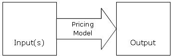
Figure 1
We can expand the ‘inputs’ box as shown below in Figure 2.
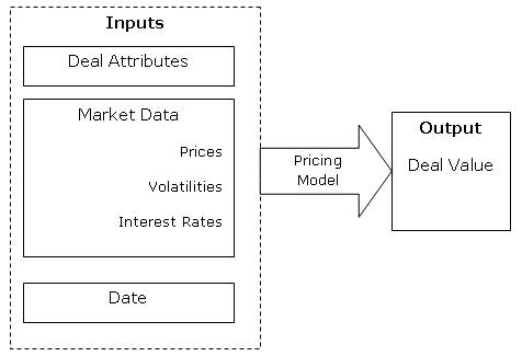
Figure 2
The inputs to the pricing model could themselves have inputs…. as shown in Figure 3 below.
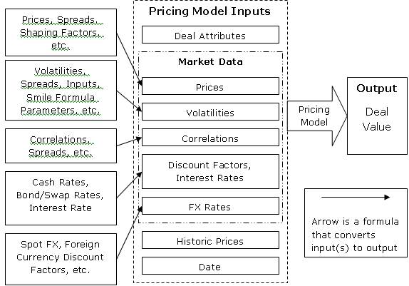
Figure 3