|
|
|


|
Main
Page by Topic |
||
|
C.
Statistics |
||
Historic
VaR
Overview
This page
covers a more details about Historic VaR.
For a general
VaR ‘Value-at-Risk’ introduction, click on this link:
Outline
2) Example
3) Ways to Calculate ‘Price Changes’
4) Considerations for CTRM Design
Historic VaR
is one of the methodologies for calculating a VaR value. A VaR value is one measure of market risk,
which we’ll define as ‘the threshold where you are expected to lose more than
that threshold just 5% of the time’.
Historic VaR
uses actual prices, i.e., commodity prices in this case. E.g., prices over a certain time frame
leading up to today. This makes Historic
VaR relatively easy to add to a CTRM system since we can assume historic settle
(‘closing’) prices would already be loaded into the system, as they are needed
to calculate index based (‘floating’) payments.
2) Example
For our
example, we’ll assume one trade of long 1000 BBL of Crude Oil. The current market price, as of 06-Jun-2019
is $52.13, which gives up a value of 1000 BBL * $52.13 = $52,130.
We’ll use
approximately 2 months of prices in our example. We’ll use 41 days of
prices. This is business days, so no
weekends or holidays.
And we’ll
follow these steps:
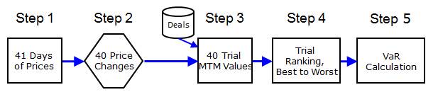
2.1) Step 1
Step 1 is to
gather the last 41 days of prices, which includes today, assumed to be 06-Jun-2019. Note that the prices are example and not real
settle prices for Crude Oil. We show an
abbreviated set of prices below, with the middle section cut out, just to make
this blog post smaller.
We count today
as ‘1’ and then count back to 41 days.
|
Day# |
Date |
Price |
|
41 |
11-Apr-2019 |
52.13 |
|
40 |
12-Apr-2019 |
52.41 |
|
39 |
15-Apr-2019 |
52.57 |
|
38 |
16-Apr-2019 |
52.75 |
|
... |
... |
... |
|
4 |
3-Jun-2019 |
52.71 |
|
3 |
4-Jun-2019 |
52.43 |
|
2 |
5-Jun-2019 |
51.90 |
|
1 |
6-Jun-2019 |
52.13 |
2.2) Step 2
For Step 2, we
calculate the price changes.
Note that we
wind up with just 40 price changes, i.e., one less than the number of
days. We used just the simple price
change of one day minus the prior day.
|
Day # |
Date |
Price |
Price Change |
|
41 |
11-Apr-2019 |
52.13 |
N/A |
|
40 |
12-Apr-2019 |
52.41 |
0.28 |
|
39 |
15-Apr-2019 |
52.57 |
0.16 |
|
38 |
16-Apr-2019 |
52.75 |
0.18 |
|
... |
... |
... |
... |
|
4 |
3-Jun-2019 |
52.71 |
0.05 |
|
3 |
4-Jun-2019 |
52.43 |
-0.28 |
|
2 |
5-Jun-2019 |
51.90 |
-0.53 |
|
1 |
6-Jun-2019 |
52.13 |
0.23 |
We can take
these price changes and rank them from worst to best. As shown in the table below.
For ‘Ranked
#’, that is based on a numbering based on the price change ranking. We kept the Day # and Date from the prior
table for a comparison, though we don’t really need those values in the
calculations going forward. Same for
showing ‘Price’, i.e., we are showing it for clarity, but we no longer need the
price. All we need is the price change.
For 95%
confidence level VaR, we want the 5% worst value, which is the row at rank 38,
which is -0.24.
So just from
this, we can say that ‘worst case’ (defined at a 5% threshold), the market
might go down -$0.24, so our 1000 BBL could go down $0.24 and so we could lose
$240. However, we’ll continue with the
other steps for clarity and, especially, because in a real situation, we won’t
just have one deal, so it will require more effort than we can just figure out
with intuition.
|
Ranked # |
Day # |
Date |
Price |
Price Change |
|
40 |
2 |
5-Jun-2019 |
51.90 |
-0.53 |
|
39 |
3 |
4-Jun-2019 |
52.43 |
-0.28 |
|
38 |
16 |
16-May-2019 |
52.93 |
-0.24 |
|
37 |
7 |
29-May-2019 |
52.42 |
-0.24 |
|
... |
... |
... |
... |
... |
|
4 |
27 |
1-May-2019 |
52.87 |
0.23 |
|
3 |
26 |
2-May-2019 |
53.1 |
0.23 |
|
2 |
1 |
6-Jun-2019 |
52.13 |
0.23 |
|
1 |
40 |
12-Apr-2019 |
52.41 |
0.28 |
2.3) Step 3
Calculate the
40 trial MTMs
For this one
deal, the new MTMs are just quantity * price.
The ‘price’ is
the ‘Trial Price’, which is the current market price and then add in the set of 40 price changes.
Looks like
this. Note that we aren’t showing these
rows ranked from best to worst. We went
back to showing rows sorted by date.
|
Day # |
Date |
Starting Price |
Price Change |
Trial Price |
Volume |
Trial MTM |
|
40 |
12-Apr-2019 |
52.13 |
0.28 |
52.41 |
1000 |
$ 52,410 |
|
39 |
15-Apr-2019 |
52.13 |
0.16 |
52.29 |
1000 |
$ 52,290 |
|
38 |
16-Apr-2019 |
52.13 |
0.18 |
52.31 |
1000 |
$ 52,310 |
|
37 |
17-Apr-2019 |
52.13 |
-0.11 |
52.02 |
1000 |
$ 52,020 |
|
... |
... |
... |
... |
... |
... |
... |
|
4 |
3-Jun-2019 |
52.13 |
0.05 |
52.18 |
1000 |
$ 52,180 |
|
3 |
4-Jun-2019 |
52.13 |
-0.28 |
51.85 |
1000 |
$ 51,850 |
|
2 |
5-Jun-2019 |
52.13 |
-0.53 |
51.60 |
1000 |
$ 51,600 |
|
1 |
6-Jun-2019 |
52.13 |
0.23 |
52.36 |
1000 |
$ 52,360 |
2.4) Step 4
Now we’ll rank
the trials by MTM, best to worst.
For this
example with just one deal, this is the same as just looking at the price
changes on their own. However, for more
complicated examples, especially with options (option trades, e.g., calls/puts), you need to look at the MTM values as they won’t directly
correlate with price changes.
|
Ranked # |
Day # |
Date |
Trial MTM |
|
40 |
2 |
5-Jun-2019 |
$ 51,600 |
|
39 |
3 |
4-Jun-2019 |
$ 51,850 |
|
38 |
16 |
16-May-2019 |
$ 51,890 |
|
37 |
7 |
29-May-2019 |
$ 51,890 |
|
... |
... |
... |
... |
|
4 |
27 |
1-May-2019 |
$ 52,360 |
|
3 |
26 |
2-May-2019 |
$ 52,360 |
|
2 |
1 |
6-Jun-2019 |
$ 52,360 |
|
1 |
40 |
12-Apr-2019 |
$ 52,410 |
2.5) Step 5
To calculate
VaR at the 95% level, we’ll take the unchanged MTM, which was $52,130 and
compare it to the MTM from the ‘worst cast’ trial MTM at the 95% level (or 5%
level going the other way), which is shown above at ‘Ranked #’ 38, or $51,890.
This given a
Historic VaR value of $240 = $52,130 - $51,890.
Some readers
may be screaming (internally) about the example using price changes based on
subtracting two days of prices and may be thinking, wouldn’t percentage changes
be better?
Indeed they
would be in many cases.
Another method
is to use the log of the percent change, i.e. the natural log. Excel has this formula as ‘ln’. There are good theoretical reasons to use
natural log and it relates to a modelling assumption that commodity price
*changes* (i.e., not prices) are lognormally distributed.
Here is the
original price changes table with extra columns for price change as a percent
and the log of the price change as a percent.
We show ‘price
change as a percent’ as 1.0053712, i.e., the new price is 100.53712% of the
prior percent. This is called the ‘one plus’ format for the price change, i.e., instead of just
saying ‘up 0.53712%’ (because we add one).
For taking the log, you need to take the log of the ‘one plus’ return.
|
Day# |
Date |
Price |
Price Change |
Price Change % |
Price Change ln
% |
|
41 |
11-Apr-2019 |
52.1 |
|
|
|
|
40 |
12-Apr-2019 |
52.4 |
0.28 |
1.0053712 |
0.0053568 |
|
39 |
15-Apr-2019 |
52.6 |
0.16 |
1.0030529 |
0.0030482 |
|
38 |
16-Apr-2019 |
52.8 |
0.18 |
1.0034240 |
0.0034182 |
|
... |
... |
... |
... |
... |
... |
|
4 |
3-Jun-2019 |
52.7 |
0.05 |
1.0009495 |
0.0009490 |
|
3 |
4-Jun-2019 |
52.4 |
-0.28 |
0.9946879 |
-0.0053262 |
|
2 |
5-Jun-2019 |
51.90 |
-0.53 |
0.9898913 |
-0.0101602 |
|
1 |
6-Jun-2019 |
52.1 |
0.23 |
1.0044316 |
0.0044218 |
When
calculating the trial MTM values, i.e., ‘shocking’ the prices based on the
price changes, you need to be consistent.
So, for example, if you calculated the price change as a percent, you
need to ‘shock’ the prices up by a percent, and if you calculated the price
changes as a subtraction from the prior day, you need to add/subtract the price
changes to the current prices to calculate your trial MTM values.
4) Considerations
for CTRM Design
The ‘Value at
Risk’ post has some important considerations for CTRM design for VaR in
general, such as ‘show your work’ and the ability to simultaneously run 95%
confidence level VaR and 99% confidence level VaR.
This section
covers some extra considerations for Historic VaR.
4.1) For each
‘price index’, CTRM systems should be able to let users decide which of three
above price change calculation approaches will be used.
4.2) Moveover, CTRM systems should allow for Historic VaR to be
run with two or more price approaches at the same time. For example, a firm might want to run VaR using
price changes based on subtracting two days (as shown in the above example) and
as a percentage change. Meaning, without having to change global system settings.
This generally
wouldn’t be needed for daily production use, but it can help during test
phases.
This is the
kind of thing that can be easy to apply to CTRM system design upfront, but,
with a bad design, can be hard to change later, i.e., after everything is
already built. So best
to get the design right upfront.
4.3) Holiday schedule handling. How
should the system handle days of missing prices. For example, suppose you have metal prices
from a London exchange, which would not post (i.e., provide prices) on a London
holiday, and crude oil prices from a New York exchange, which would not post
prices on a New York holiday, e.g., Fourth of July. The system needs to handle that
4.3.1) Correctly, meaning the numbers are as desired (and not
necessarily just one ‘correct’ way, i.e., correct is in the eye of the
beholder).
4.3.1.1) E.g.
first you need, for Historic VaR to be accurate, to line up all ‘trial MTMs’ by
the date. That could be the union of all
days that are a good business date for any one pricing source. Or maybe best to have a specific holiday
calendar, separately maintained, for which are considered the good business
days for the firm for calculating Historic VaR (i.e., rather than have the
system try to figure it out on its own based on when prices were published).
4.3.2) In a transparent way (i.e., ‘show your work’).
4.3.3) Giving
the user options, i.e., choices on how to handle the missing prices. An interpolation method. Example: If London publishes July 1, 2, 3, 4, and 5th
(five prices) and New York publishes July 1, 2, 3, and 5 (four prices, no price
on the holiday), the historic VaR framework would come up with an interpolated
price for July 4. This should be based
on however the user wants it work. E.g., average of the prices for the 3rd and 5th? Or ‘backstep’
interpolation, which is just to copy the prior day’s price, i.e., use the price from the 3rd as the New York price
for the 4th.
Introduction to
CTRM
Click on this
link for a great introduction to CTRM software: Introduction to CTRM Software